Another Oddball System

(developed by Mark Brown www.markbrown.com)

Market: Futures

System Concept 

This month’s article is a reality check on a futures system that was published on a public forum in 1997 by Mark Brown, a well-known personality in the trading system industry. According to his statement he had traded it (or similar systems) for many years and has since moved on to other system trading styles. In his introductory comment for this system he made the following interesting statement:

“It's as much a mind game as anything and if you want to make money let your mind go blank and trust the system, the system can be intuitive or computerized or any blend thereof. But defined and cast in stone it must be.”

According to the method, we create a 38 bar, 3 standard deviation Upper Bollinger Band of the 10 bar Adaptive Moving Average of high prices, and a corresponding Lower Band of low prices. The Adaptive Moving Average is taken from Perry Kaufmann, whose Adaptive Moving Average (AMA) automatically increases the speed of the moving average as market volatility increases.   

The entry and exit rules are rather straightforward.  When the closing price crosses above the upper band we go long, and below the lower band we go short.  Since the published methodology defines only the entry and exit rules, we have added our own position sizing rules, which are summarized below.  As the system is trend-following in nature and is “always in” the market (later we’ll see that this is not the precisely the case due to the effect of our self-imposed position sizing rules), it is expected to work best in trending, non-correlated markets and is therefore ideal for our Active Trader magazine sample portfolio. 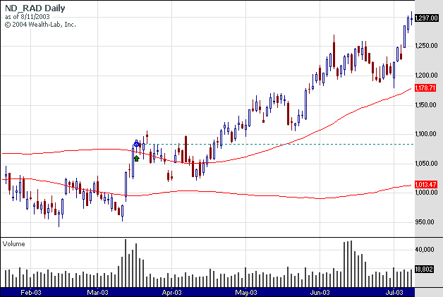Figure 1 shows an sample trade.

Entry and Exit Rules 

1. Construct Bollinger Bands based on a 10 bar Adaptive Moving Average of highs and lows.
2. Go long and cover a short position on the next bar’s open when closing price crosses above the top band.
3. Go short and sell a long position on the next bar’s open when closing price prices crosses below the bottom band.

Portfolio Simulation Settings 

1. Starting equity is $250,000.
2. Risk a maximum of 1% of total account equity per trade (stop-based Risk %) to calculate the number of contracts.
3. Deduct $10 slippage/commission per contract (entry and exit).

Test Data

The system was tested on the Active Trader Standard Futures Portfolio, which contains the following 20 futures: DAX30 (AX), Corn (C), Crude Oil (CL), German Bund (DT), Euro Dollar (ED), Euro Forex (FX), Gold (GC), Copper (HG), Japanese Yen (JY), Coffee (KC), Live Cattle (LC), Live Hogs (LH), NASDAQ100 (ND), Natural Gas (NG), Soybeans (S), Sugar (SB), Silver (SI), S&P 500 (SP) and T-Notes 10 year (TA). For this article we used Ratio Adjusted data from Pinnacle Data Corp. 

Test Period: June 1997 until August 2003 (out of sample data) 

Money Management 

Often money management is also referred to as position sizing, portfolio allocation and so on. Proper money management defines two important and related rules: position sizing and the bet sizing. Bet sizing defines which percentage of the portfolio’s total equity the trader is willing to risk (to bet). The position size calculates how many contracts the trader should open on any given trade expecting the worst outcome (stop loss triggered). The number of contracts is calculated using a basis price, the stop loss level, the contract’s point, and the portfolio’s total equity.  The basis price is the price at which the market closes prior to putting on a new position.   

Using an example of a commodity with a point value of $250, assume that the entry signal goes long at a basis price of $100 and the stop loss on that date is shown to be at $90.  We calculate our dollar risk by multiplying $250 by $10 ($100 - $90).  Consequently, if we were stopped out on the purchase of one contract, we would lose $2,500. Now, if our portfolio’s total equity on the date before entering into the position was at $320,000, and we do not want to risk more than one percent of our total equity ($3,200), we would be allowed to buy one contract since the integer part of the quotient $3,200/$2,500 is 1. Had total equity been below $250,000, we would not be able to take this position since the dollar risk would exceed the 1% equity risk that we are willing to assume. 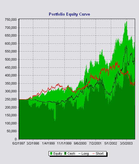This position sizing method keeps us out of risky trades that have potential to ruin our account, and in the same way, it keeps us from entering other markets entirely since the risk is too high during specific trading periods. In Figure 2 we show the result of the system when risking one percent of the total portfolio equity per trade.  

System Results 

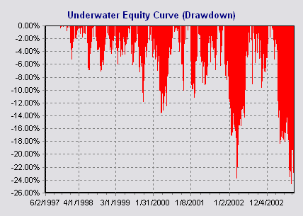
With $250,000 of starting capital, the system achieved an overall profit of 129.99% in approximately six years and accomplished an average annual return of 13.78 percent, with the worst year being a loss of 13.20 percent in 2003. The same year had the largest drawdown of 26.01 percent. Out of 251 trades, only 31.08 percent were winners.  Nevertheless, the average profit per trade was $1,294.76. Over our testing period, trading from either side, long or short, was profitable and complementary as you can quickly observe by the thin red and black lines (equity curves attributable to short and long trades, respectively) in Figure 2, the portfolio equity curve. Even thou this is essentially a stop and reverse (SAR) system, we can see a rather moderate exposure of 33.79% which would give us some room to increase risk.  

Effect of Money Management 

To demonstrate the effect of money management on overall system performance, we now double the risk per trade to two percent of total portfolio equity. Looking at the same system with the increased risk, Figure 3 illustrates an equity curve with much greater volatility accompanied by higher draw downs (45% compared to the earlier 26%) and even less profit (42% compared to the earlier 129%). Exposure climbs to over 37%, and the number of trades reduces to 237 due to the fact that at certain periods insufficient equity existed to assume the 2% programmed risk.  

Conclusion 

Given that the system was published free of charge and we have not changed any parameters, it shows a rather good result. We did not make any market selection as it was not stated for which market it was created. Many commercial systems are often optimized for certain markets. On the other hand, there is no guaranty that the market “character” will stay the next ten years as it was the last ten years. Diversification and sound money management is the key to success as many hedge fund managers are proving year after year. The more markets you can trade, the more likely you will catch the big trend that those systems require to be profitable. The pure fact that this trading system was offered gratis does not make it a better or worse than others. Each trader should fully evaluate and research any system before risking real money. 

Strategy Summary

LEGEND: Net Profit – Profit at end of test period, less commission · Exposure – The area of the equity curve exposed to long or short positions, as opposed to cash · Profit Factor – Gross Profit divided by Gross Loss · Payoff Ratio – Average Profit of Winning Trades divided by Average Loss of Losing Trades · Recovery Factor – Net Profit divided by Max Drawdown · Max DD% - Largest percentage decline in Equity · Longest Flat Days – Longest period, in days, the system is between two Equity highs · No. Trades – Number of trades generated by the system · Win/Loss% - The percentage of trades that were profitable · Avg. Profit – The average profit for all trades · Avg. Hold Time – The average holding period for all trades · Avg. Profit (Winners) – The average profit for winning trades · Avg. Hold Time (Winners) – The average holding time for winning trades · Avg. Loss (Losers) – The average loss for losing trades · Avg. Hold Time (Losers) – The average holding time for losing trades · Max Consec.. Win/Loss – The maximum number of consecutive winning and losing trades 

Periodic Returns

LEGEND: Avg. Return – The average percentage for the period · Sharpe Ratio – Average return divided by standard deviation of returns (annualized) · Best Return – Best return for the period · Worst Return – Worst return for the period · % Profitable Periods – The percentage of periods that were profitable · Max Consec.. Profitable – The largest number of consecutive profitable periods · Max Consec. Unprofitable – The largest number of consecutive unprofitable periods. 

Sample Trade

Notice how the bands expand with the increased volatility.

Equity Curve 1%

The equity curve with the 1% money management rule applied.

Drawdown

The underwater equity curve of the system when applying the 1% equity risk money management rule.

MetaStock code:

To create the system test, open the tester under the Tools menu. Select new test and enter the following formulas in for the specific orders.

Enter Long:
ama:=If(Cum(1)=5,Ref(C,-1)+(Pwr((Abs((C-Ref(C,-4))
/Sum(Abs(ROC(C,1,$)),4)))*((2/3)-(2/31))+(2/31),2))*
(C-Ref(C,-1)),PREV+(Pwr((Abs((C-Ref(C,-4))
/Sum(Abs(ROC(C,1,$)),4)))*((2/3)-(2/31))+(2/31),2))*(C-PREV));
C>BBandTop(ama,38,S,3)

Close Long:
ama:=If(Cum(1)=5,Ref(C,-1)+(Pwr((Abs((C-Ref(C,-4))
/Sum(Abs(ROC(C,1,$)),4)))*((2/3)-(2/31))+(2/31),2))*
(C-Ref(C,-1)),PREV+(Pwr((Abs((C-Ref(C,-4))
/Sum(Abs(ROC(C,1,$)),4)))*((2/3)-(2/31))+(2/31),2))*(C-PREV));
C<BBandBot(ama,38,S,3)

Enter Short:
ama:=If(Cum(1)=5,Ref(C,-1)+(Pwr((Abs((C-Ref(C,-4))
/Sum(Abs(ROC(C,1,$)),4)))*((2/3)-(2/31))+(2/31),2))*
(C-Ref(C,-1)),PREV+(Pwr((Abs((C-Ref(C,-4))
/Sum(Abs(ROC(C,1,$)),4)))*((2/3)-(2/31))+(2/31),2))*(C-PREV));
C<BBandBot(ama,38,S,3)

Close Short:
ama:=If(Cum(1)=5,Ref(C,-1)+(Pwr((Abs((C-Ref(C,-4))
/Sum(Abs(ROC(C,1,$)),4)))*((2/3)-(2/31))+(2/31),2))*
(C-Ref(C,-1)),PREV+(Pwr((Abs((C-Ref(C,-4))
/Sum(Abs(ROC(C,1,$)),4)))*((2/3)-(2/31))+(2/31),2))*(C-PREV));
C>BBandTop(ama,38,S,3)

inputs:BBLength(38),BBStdDev(3),
BBHPrice(ADAPTIVE(H,10)),BBLPrice(ADAPTIVE(L,10));

vars:BBH(0),BBL(0);

BBH=BollingerBand(BBHPrice,BBLength,BBStdDev);
BBL=BollingerBand(BBLPrice,BBLength,-BBStdDev);

if c >bbh then buy;
if c<bbl then sell;

{
P.S. The adaptive function part is Perry Kaufmans:
}
inputs:price(numericseries),period(numericsimple);

vars: noise(0),signal(0),dif(0),efratio(0),
       smooth(1),fastend(.666),slowend(.0645),am(0);

{CALCULATE EFFICIENCY RATIO}
dif=@AbsValue(price - price[1]);
if(currentbar <= period) then am =price;
if(currentbar > period)then begin
        signal = @AbsValue(price - price[period]);
        noise = @summation(dif,period);
        efratio = signal/noise;
        smooth = @Power(efratio*(fastend - slowend) + slowend,2);

{ADAPTIVE MOVING AVERAGE}
       am = am[1] + smooth*(price - am[1]);
     Adaptive=am;
        end;